If you have spent any time in the machine learning space, you have inevitably scratched your head around the concept of backpropagation.
It is the undisputed engine of neural networks, and where the mathematical brain that allows a model to actually learn from its mistakes actually lives.
But for many of us, backpropagation can be hard to understand at first. Then it sort of makes sense, but as Einstein said, “If you can’t explain it simply, you don’t understand it.”
We are faced with the chain rule, partial derivatives, and gradient descent, and told to just trust the math.
While the math is elegant, it often obscures the intuitive, mechanical reality of what is actually happening inside the network.
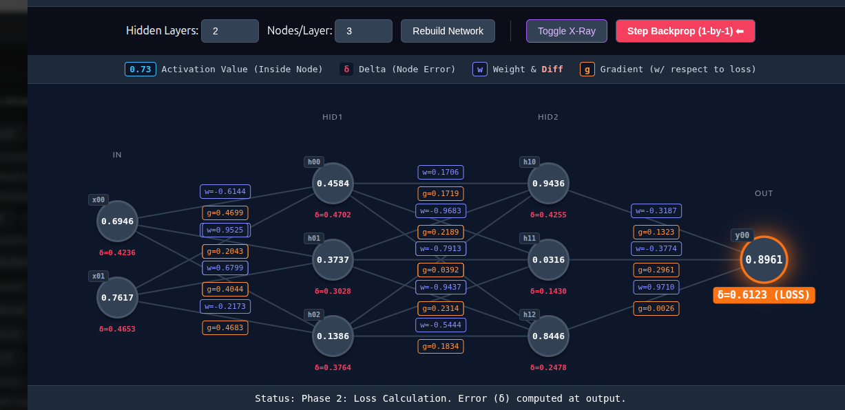
I wanted to bridge that gap between abstract equations and visual intuition, so I could explain it simply, therefore I built an Interactive X-Ray Neural Network Visualizer.
Click the button to launch it:
The “Responsibility Game” – who’s to blame for the error?
Instead of treating the network like a black box, this visualizer slows down time and exposes the raw mechanics of a neural network. It breaks the learning cycle into individual, step-by-step phases so you can watch the math unfold in real-time.
Here is exactly what it reveals:
- The Forward Pass: You watch the input signal cascade through the network. At each node, you see the exact activation value (a) being calculated and passed along the connections.
- Calculating the Loss: Once the network makes its guess, it compares it to the target. The visualizer instantly calculates the error, quantifying exactly how wrong the network was.
- The Backward Pass (The Responsibility Game): This is where the magic happens. The network goes in reverse, calculating the delta (δ) for each node. It essentially asks, “How much is this specific node to blame for our final error?” You can watch the error propagate backward, layer by layer.
- Updating the Weights: For every connection, the visualizer calculates the gradient (g)—the exact directional step needed to fix the mistake. When the weights (w) update, the interface highlights the precise change (e.g.,
w: 1.25 ➔ 1.10), showing you the network physically adjusting itself to make a better guess in the next round.
By exposing the activations, deltas, weights, and gradients right on the connections, backpropagation can be undrstoon n practical terms.
It becomes something much simpler to grasp: a system of components playing a massive game of responsibility, tweaking their dials step-by-step until they arrive at the right answer.
Let me know if this is as helpful to you as it was to me.
More on the #AI for Dummies series
Be First to Comment